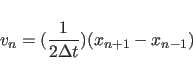
Finite Difference Approximation
X-PLOR makes use of a third-order
finite difference approximation in
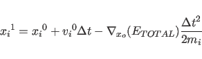
![$dt$](img294.png)
(
Brünger, Brooks, and Karplus, 1984).
First, the initial coordinates
![${x_i}^0$](img295.png)
are subjected to the SHAKE method.
Then the system gets the initial velocities
![${v_i}^0$](img296.png)
. Next,
the program prints the energy of the initial coordinates. A two-step
method is used to obtain the coordinates
![${x_i}^1$](img297.png)
:
![\begin{displaymath}
{x_i}^1 = {x_i}^0 + {v_i}^0 \Delta t -
{\nabla}_{x_o}(E_{TOTAL}) {{\Delta t}^2 \over 2 m_i}
\end{displaymath}](img298.png) |
(11.8) |
IF SHAKE constraints are present,
the SHAKE method is applied to
![${x_i}^1$](img297.png)
with respect to
![${x_i}^0$](img295.png)
.
Iteration from step
to step
causes
.
The algorithm computes the forces
.
The algorithm then computes
![\begin{displaymath}
x_i^{n+1} = [1 + {b_i \Delta t \over 2}] ^{-1} [ 2 x_i^n - x...
...Delta t}^2 \over m_i} + x_i^{n-1} ({b_i {\Delta t} \over 2}) ]
\end{displaymath}](img302.png) |
(11.9) |
If required, the SHAKE method
is applied to
![$x_i^{n+1}$](img303.png)
with
![$x_i^n$](img304.png)
as the
reference set. Finally, the velocities at this step are computed:
![\begin{displaymath}
v_n = ( {1 \over 2 \Delta t} ) ( x_{n+1} - x_{n-1} )
\end{displaymath}](img305.png) |
(11.10) |
(The velocities do not enter the equations to compute the
trajectory
![$x_i^n$](img304.png)
.) In case of
zero friction coefficients
![$b_i$](img283.png)
, this algorithm
reduces to the three-step Verlet method
(
Verlet, 1967).
Xplor-NIH 2024-09-13